Borrowing a tool from systems biology for mechanistic interpretability

TL;DR: I have been analyzing attribution graphs manually and found it to be tedious and hard to scale. To help automate some of this process, I ported network motif analysis (the technique Uri Alon used to decode gene regulatory networks) into a tool for automatically fingerprinting the structural properties of transformer circuits. I ran it on 99 attribution graphs from Neuronpedia. The graphs are dominated by feedforward loops (FFLs), confirming that the tool recovers structure that Anthropic had previously observed qualitatively in individual circuits. The more interesting results are: (1) when I trace individual FFLs in a concrete circuit, they chain into multi-stage processing cascades with interpretable roles like grounding, entity resolution and output competition via inhibitory edges. And (2), the motif profiles show a consistent structural backbone across all task types but have with task-specific differences in the magnitude of individual motifs. The tool (circuit-motifs) is open source and runs on any attribution graph from Neuronpedia.

Staring into the abyss (attribution graph)

On a Youtube video called “Attribution Graphs for Dummies,” put out by researchers at Anthropic, DeepMind and Goodfire AI, Emmanuel Ameisen states at the beginning that he has spent so much time staring at attribution graphs that he now believes they are useful. In my own experience of staring, I have come to a similar conclusion and my eyes are starting to hurt. Attribution graphs, directed graphs where nodes are features and edges represent causal influence between them [1, 2], have become an important tool in mechanistic interpretability since Anthropic’s circuit tracing work in early 2025. However, analyzing them is mostly manual and involves researchers visually inspecting node clusters so they can trace paths, group features into supernodes and build intuitions about circuit structure one graph at a time. And this is only for looking at how the model decided to say a single output token.

A recent multi-organization review of the circuits research landscape [3] flagged two open problems. First, can the process of analyzing attribution graphs be “made more systematic or even automated”? Second, can we move beyond the “local” per-prompt picture to “obtain a more global circuit picture” by aggregating across many graphs?

Network motif analysis from systems biology can potentially help with both. The technique, introduced by Milo et al. in 2002 [4], counts small recurring connectivity patterns in a network and compares observed counts to a null model. This produces a structural fingerprint (a vector of Z-scores) that characterizes the network’s wiring. The same approach that helped reveal the computational building blocks of E. coli transcription networks [5, 6] and enabled Milo et al. to classify networks from entirely different domains into structural “superfamilies” [7] can be applied directly to attribution graphs.

Anthropic’s interpretability program leans heavily on the biological metaphor as their featured paper is titled “On the Biology of a Large Language Model” [2], and Lindsey et al. explicitly identified feedforward loops in their circuits. I am to take the biology metaphor further by applying a quantitative framework from systems biology to 99 graphs (problems?) with the goal of learning about the model’s aggregate structural grammar.

Network motifs

The basic idea behind network motifs is to count all instances of small subgraphs in a network and then compare the counts to a group of randomized networks that preserve basic properties like degree distribution. Based on this comparison, you can determine which patterns appear significantly more or less often than chance. The theory is then that enriched motifs indicate functional building blocks and depleted motifs represent configurations the system actively avoids [8].

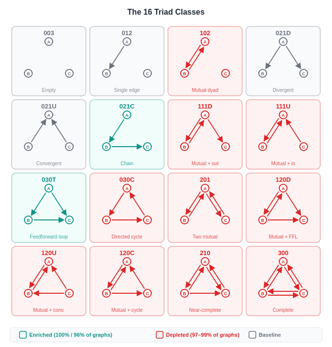
For directed networks, we can run a triad census [9] which looks for all of the 16 possible 3-node directed subgraphs. After this, each network gets a vector of Z-scores (aka motif profile) that serves as a structural fingerprint. The approach has been successfully applied to fields from neural connectivity to electronic circuits [7].

The graphs

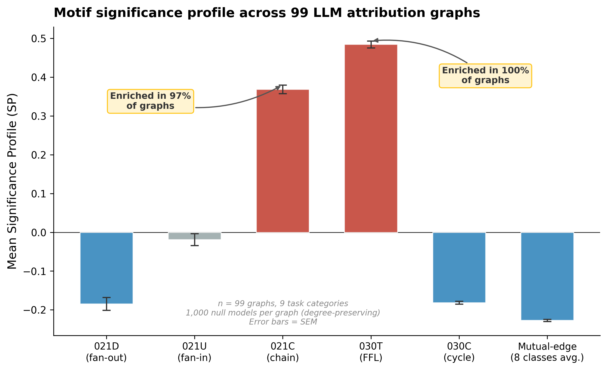
To test out the tool, I took 99 attribution graphs from Neuronpedia [11] and ran a full census on each one (with 1000 random re-wirings per graph). These graphs are produced by Anthropic’s circuit tracing methodology which replaces a model’s MLP layers with interpretable sparse coding components (transcoders) and traces causal influence between the resulting features [1]. The graphs contain 9 task categories (math, code, creative writing, fact recall, multihop reasoning, multilingual, logical reasoning, safety, and uncategorized), ranging from 24 to 433 nodes and 82 to 31,265 edges.

Since raw Z-scores scale with network size, comparison requires normalization. To address this, I use the significance profile (SP) [7] which converts the Z-score vector to a unit vector and isolates the shape of the motif signature from its magnitude (see Appendix).

The enriched motifs

030T — the feedforward loop (FFL): Enriched in 100% of graphs, with a mean Z-score of +25.7 and a maximum of +63.5. This is the pattern where A influences C directly and also indirectly through B. And it is the “coherent feedforward loop” that Lindsey et al. [2] identified in their Dallas→Texas→Austin circuit:

Convergent paths and shortcuts. A source node often influences a target node via multiple different paths, often of different lengths. [...] In the taxonomy of Alon, this corresponds to a “coherent feedforward loop,” a commonly observed circuit motif in biological systems.

021C — the two-path cascade: Enriched in 97% of graphs (mean Z = +19.8). The simplest feedforward chain with a shared intermediary where A sends to both B and C.

All the other motifs were depleted. The five core mutual-edge motifs (111D, 111U, 120D, 120U, 120C) are significantly depleted in 99-100% of graphs (mean Z-scores −15 to −17). The remaining mutual-edge motifs (201, 210, 300) are depleted in 64-94% of graphs. The directed three-cycle (030C) is depleted in 98% of graphs. The actual count of three-node directed cycles across all 99 graphs is zero.

This makes sense. The residual stream flows forward in a transformer so cycles should not appear. The FFL enrichment is consistent with the convergent multi-path structure Anthropic observed in individual circuits but is now quantified across 99 graphs. A mean Z of +25.7 means this convergent structure is much stronger than what degree distribution alone would predict.

Size, architecture and model effects

Before moving on, we should talk about three potential factors that could confound these results I tried to account for (see appendix for the full analysis):

Graph size. Raw Z-scores correlate with edge count (Spearman r = +0.86, p < 0.0001), but after SP normalization [7], the correlation goes away (r = -0.02, p = 0.81). All cross-task comparisons below use SP-normalized values.

Transcoder architecture. I compared motif profiles for 21 matched prompt pairs traced with both cross-layer transcoders (CLTs) and per-layer transcoders (PLTs) on Claude Haiku. The overall profile shape is consistent (cosine similarity = 0.981), though the dominant motif shifts: PLTs favor FFLs (SP = 0.479 vs 0.424), CLTs slightly favor chains (SP = 0.441 vs 0.384). Overall, both show the same enrichment/depletion pattern.

Cross-model generalization. Do we see significantly different motif profiles in a different model? To address this, I ran the same prompt through Claude Haiku, Gemma-2-2B, and Qwen3-4B. All three show FFL-dominated profiles. Pairwise cosine similarities range from 0.86 to 0.91. This is a single-prompt comparison, but it suggests the finding isn’t model-specific.

The tool can help find interpretable circuit traces

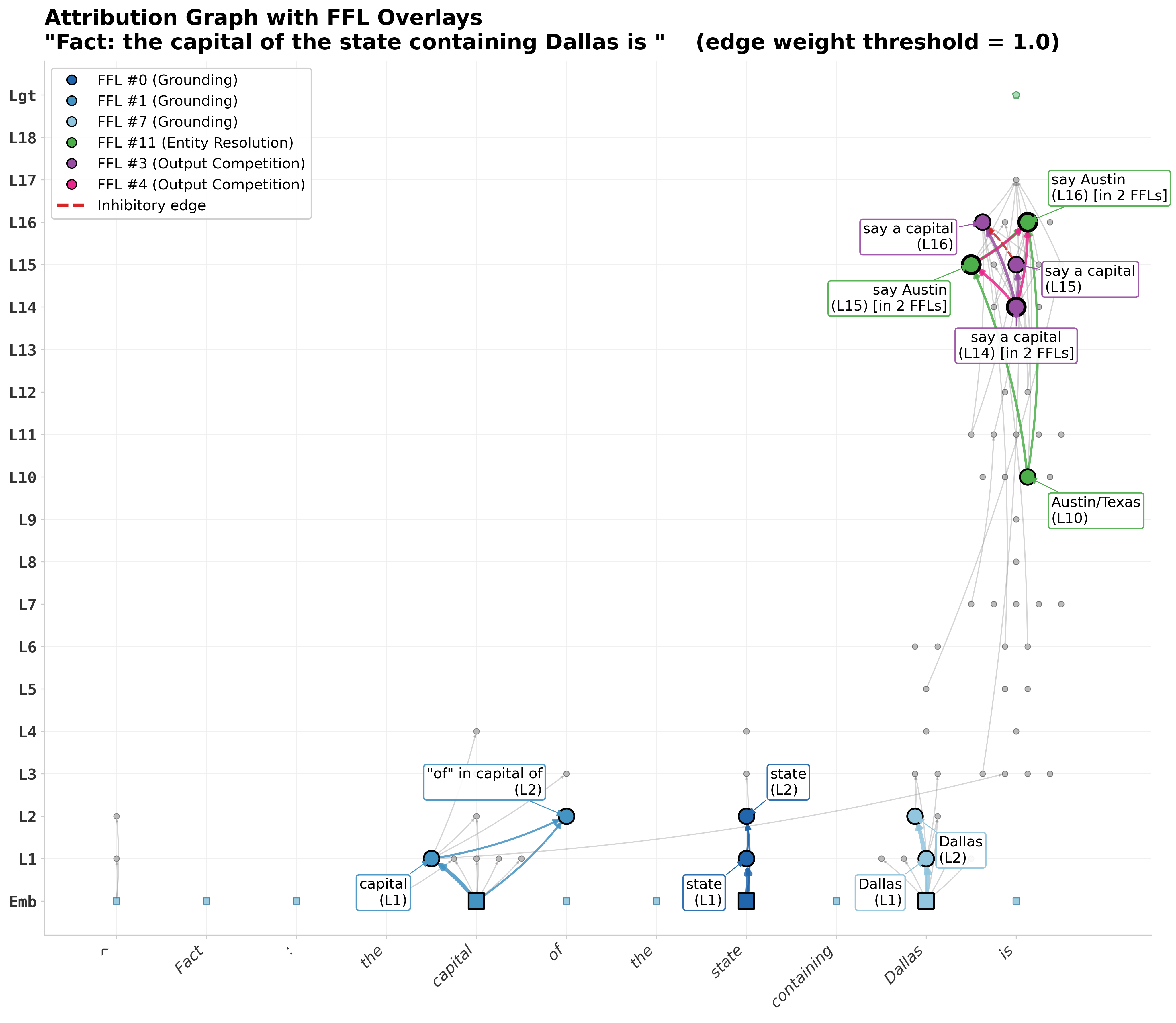
The aggregate statistics are great but what we really want is an interpretable trace to understand why the model decided to say what it said. The tool can help with this because it rapidly identifies the highest weighted FFLs and then we can inspect these to try and make sense of the model’s internal processes. To demonstrate this, I looked at some of the highest-weight FFLs in the attribution graph for a multi-hop fact recall prompt, “The capital of the state containing Dallas is _ .” I picked this prompt because it is the same prompt Lindsey et al. used as their case study [2] and the one where they first noted the coherent feedforward loop structure.

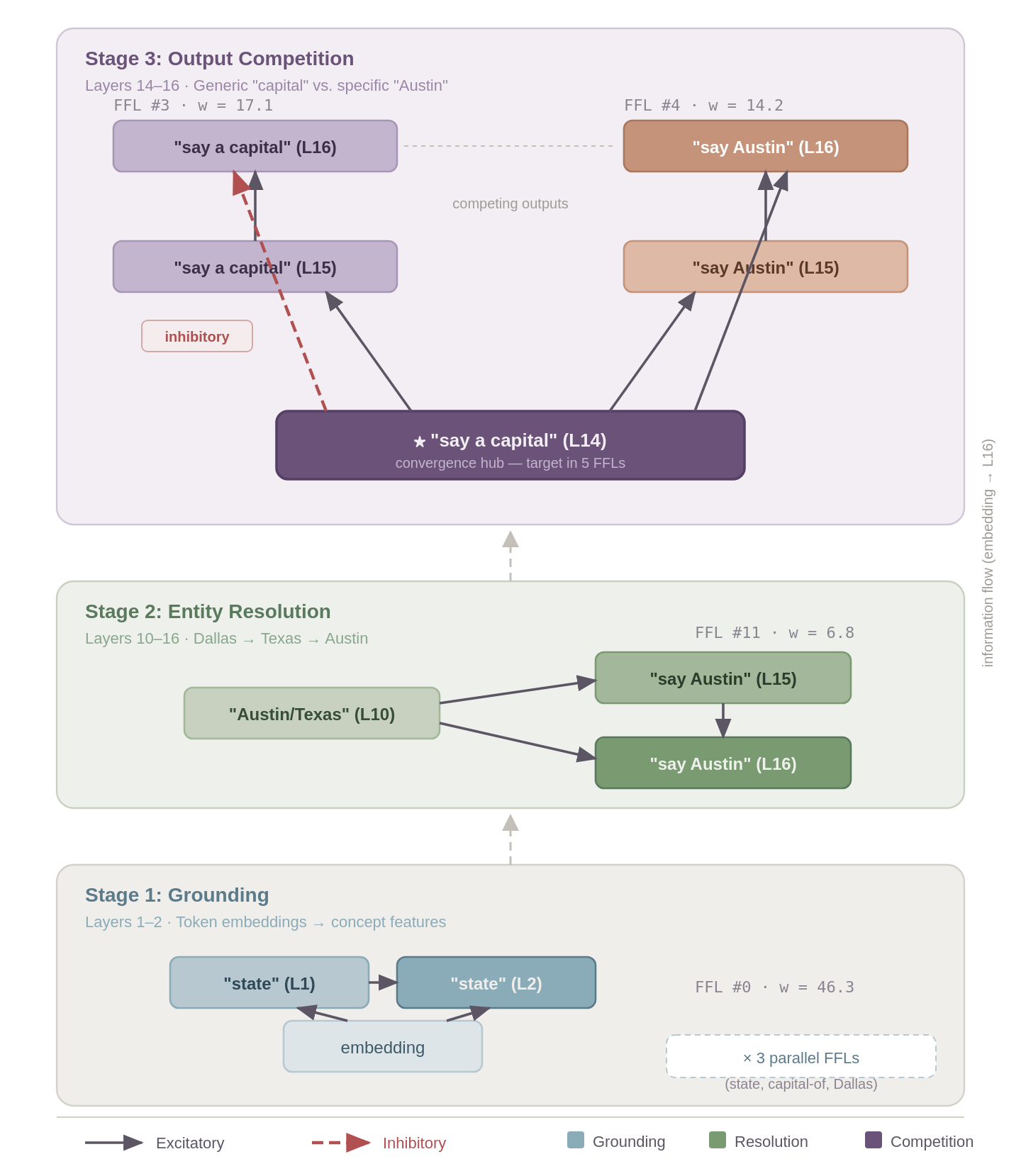
Based on the FFLs, I tried to identify different stages of processing.

Stage 1 — Grounding (Layers 1–2). Three parallel FFLs extract the key concepts from the input embeddings. FFL #0 (w = 46.3, the strongest in the entire graph) maps the token embedding for “state” through L1 and L2 features, establishing the category being queried. FFL #1 (w = 22.0) extracts the relational concept “capital of,” and FFL #7 (w = 11.3) grounds the anchor entity “Dallas.” Each of these follow the same structure where the embedding (regulator) feeds into both an L1 feature (mediator) and an L2 feature (target), with L1 also feeding L2. This represents two convergent paths from raw input to refined representation. All three are fully excitatory and operate in parallel with each establishing one piece of the reasoning puzzle.

Stage 2 — Entity Resolution (Layers 10–16). A single FFL bridges the gap between concept grounding and answer generation. FFL #11 (w = 6.8) connects an “Austin/Texas” feature at L10 to “say Austin” features at L15 and L16; the step where the multi-hop chain Dallas → Texas → Austin is resolved. This appears to be the critical reasoning step where the model has grounded both the input text structure and the anchor entity in Stage 1, and now resolves them to a specific answer.

Stage 3 — Output Competition (Layers 14–16). Two FFLs converge on a shared node, “say a capital” at L14, which serves as the target in five different FFLs across the full graph, making it a convergence hub. This is where the model decides between the generic response (”a capital”) and the specific answer (”Austin”). FFL #3 (w = 17.1) propagates the generic “capital” concept forward from L14 through L15 to L16, but its direct shortcut edge from L14 to L16 is inhibitory (the only negative-weight edge among all six FFLs). This creates a self-suppression mechanism where the generic response is partially dampened at the final layer. Meanwhile, FFL #4 (w = 14.2) channels the abstract “capital” representation at L14 into the specific entity “Austin” at L15 and L16, with all edges excitatory. The competition resolves and the correct-answer pathway is fully reinforced while the generic pathway brakes itself.

A few things jump out form this. First, the FFLs can compose. The output of one stage's FFLs becomes the input to the next, forming a processing pipeline from token embeddings to output logits. Second, the convergent dual-path structure of each FFL is analogous to the persistence-detection motif described in biological networks [5, 6] where the target only activates when evidence arrives through both paths. Whether transformer FFLs serve a similar filtering function is an open question but I think the structural similarity is notable. Third, the single inhibitory edge shows that FFLs aren't limited to signal amplification and the model can use them to suppress incorrect outputs or to push for correct ones.

Task types show consistent backbone with local modulation

All task-type pairs show high cosine similarity (0.90–0.998), reflecting the dominance of the universal FFL/chain enrichment pattern across all graph categories. A permutation test (10,000 label shuffles, corrected for 36 pairwise comparisons) confirms that no pair is significantly more similar than expected by chance and randomly grouped graphs converge toward the global mean profile even more tightly than the real task groupings do. The high absolute similarities show the graphs have a similar wiring but not task-specific clustering.

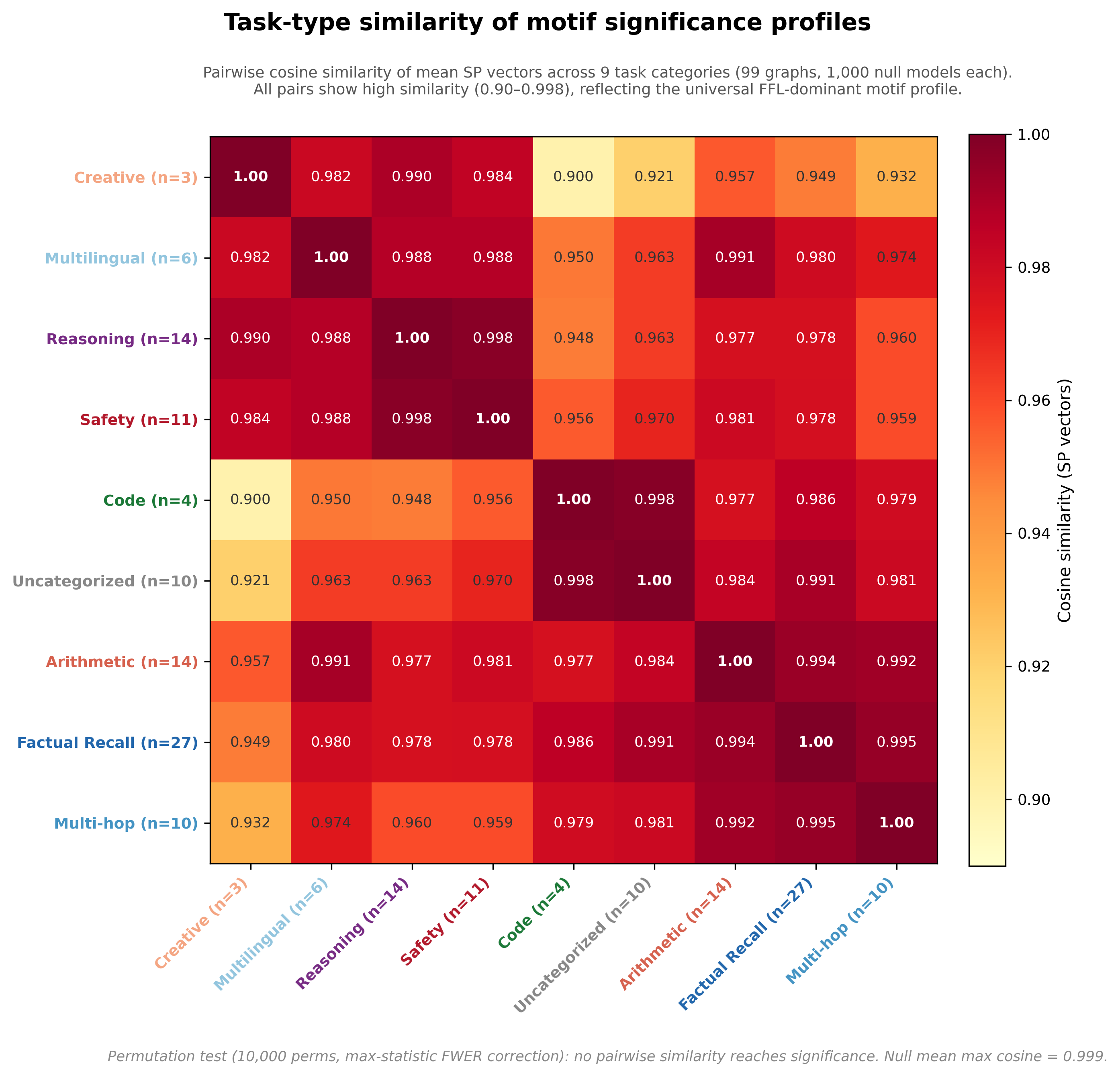
The task-type signal appears instead in per-motif magnitude differences. Kruskal-Wallis tests show that 11 of 16 motif classes have significantly different SP-normalized distributions across task categories. In other words, every task type uses the same motif vocabulary (FFL-dominant, chain-enriched, cycle-depleted) but the intensity of enrichment or depletion along individual motif dimensions varies. Maybe there is more to investigate here.

The tool and how to use it

The analysis pipeline in circuit-motifs is designed to work with any attribution graph from Neuronpedia. Given a graph, it:

1. Runs the full triad census (~seconds per graph)

2. Generates Z-scores against a degree-matched, acyclicity-preserving null model

3. Computes SP-normalized motif profiles for cross-graph comparison

4. Identifies and ranks individual motif instances by edge weight for circuit-level analysis

Citations

1. Ameisen, E., Lindsey, J., Pearce, A., Gurnee, W., Turner, N. L., Chen, B., Citro, C., et al. (2025). Circuit tracing: Revealing computational graphs in language models. Transformer Circuits Thread. transformer-circuits.pub/2025/attribution-graphs/methods.html

2. Lindsey, J., Gurnee, W., Ameisen, E., Chen, B., Pearce, A., Turner, N. L., Citro, C., et al. (2025). On the biology of a large language model. Transformer Circuits Thread. transformer-circuits.pub/2025/attribution-graphs/biology.html

3. Lindsey, J., Ameisen, E., Nanda, N., Shabalin, S., Piotrowski, M., McGrath, T., Hanna, M., Lewis, O., et al. (2025). The Circuits Research Landscape: Results and Perspectives — August 2025. Neuronpedia. neuronpedia.org/graph/info

4. Milo, R., Shen-Orr, S., Itzkovitz, S., Kashtan, N., Chklovskii, D., & Alon, U. (2002). Network motifs: Simple building blocks of complex networks. Science, 298(5594), 824–827.

5. Mangan, S. & Alon, U. (2003). Structure and function of the feed-forward loop network motif. Proceedings of the National Academy of Sciences, 100(21), 11980–11985.

6. Mangan, S., Zaslaver, A., & Alon, U. (2003). The coherent feedforward loop serves as a sign-sensitive delay element in transcription networks. Journal of Molecular Biology, 334(2), 197–204.

7. Milo, R., Itzkovitz, S., Kashtan, N., Levitt, R., Shen-Orr, S., Ayzenshtat, I., Sheffer, M., & Alon, U. (2004). Superfamilies of evolved and designed networks. Science, 303(5663), 1538–1542.

8. Alon, U. (2007). Network motifs: Theory and experimental approaches. Nature Reviews Genetics, 8(6), 450–461.

9. Holland, P. W. & Leinhardt, S. (1976). Local structure in social networks. In D. Heise (Ed.), Sociological Methodology 1976. San Francisco: Jossey-Bass.

10. Zambra, M., Maritan, A., & Testolin, A. (2020). Emergence of network motifs in deep neural networks. Entropy, 22(2), 204.

11. Lin, J. (2024). Neuronpedia: An open source interpretability platform. neuronpedia.org

Appendix

Controlling for graph size

Raw FFL Z-scores correlate strongly with edge count (Spearman r = +0.86, p < 0.0001). After SP normalization [7], the correlation vanishes entirely (r = -0.02, p = 0.81). This holds across all key motifs: raw correlations of 0.63-0.96 drop to 0.02-0.16 after normalization.

Transcoder architecture comparison

I compared 21 matched prompt pairs traced with both CLT and PLT on Claude Haiku. Overall cosine similarity = 0.981. The dominant motif shifts: in CLT graphs, the two-path chain (021C) narrowly leads the FFL in 13 of 21 graphs (mean SP = +0.44 vs. +0.42). In PLT graphs, the FFL dominates in all 21 (mean SP = +0.48 vs. +0.38). This seems to make architectural sense. CLTs span multiple layers and encode sequential flow like a chain motif. PLTs decompose each layer independently so convergent two-path structure (FFL) might be more favored. Finally, FFL and chain SP values are uncorrelated across prompts between architectures (Spearman r ≈ 0), indicating a systematic architecture effect.

Cross-model generalization

The same multi-hop prompt produces the FFL-dominant profile in Claude Haiku, Gemma-2-2B, and Qwen3-4B. The analysis produces SP values of +0.50 (Haiku), +0.46 (Gemma) and +0.72 (Qwen3-4B). And cross-model cosine similarity values of Haiku-Gemma = 0.908, Haiku-Qwen = 0.902 and Gemma-Qwen = 0.864. Even though this is a single prompt comparison, it serves as a quick check for any largely different motif profiles in different models.

Threshold sensitivity

Varying the edge-pruning threshold on the same graph produces cosine similarities of 0.84–0.99 between resulting motif profiles. Adjacent thresholds are consistent (0.87–0.99), while extreme threshold differences show more variation. The structural signature is stable across reasonable threshold choices.